|
Histogram Bin-width Optimization
Web application for optimizing a histogram |
|
Shimazaki and Shinomoto. Neural Comput, 2007,
19(6), 1503-1527 |
Web Application for Bin-width Optimization (Ver. 2.0)
|
2.
This may take some time.
*The data is processed on your own computer (the data is NOT transferred to our server). *The program searches number of bins from 2 to 200. 07/06/16 Ver. 1.0 Web Application for Histogram Bin-width
Optimization © 2006-2011 Hideaki Shimazaki
|
Histogram Binwidth Optimization Method
|
Shimazaki and Shinomoto, Neural Comput 19 1503-1527, 2007 I. Divide the data range into  and
and  * *IV. Repeat i-iii while changing *VERY IMPORTANT: Do NOT use a variance that uses N-1 to divide the sum of squared errors. Use the biased variance in the method. *To obtain a smooth cost function, it is recommended to use an average of cost functions calculated from multiple initial partitioning positions.
|
Histogram Optimization in a Nutshell
|
Original papers
|
From the observed data only, the method estimates a binwidth that minimizes expected L2 loss between the histogram and an unknown underlying density function. An assumption made here is merely that samples are drawn from the density independently each other. The method was developed in collaboration with Prof. Shinomoto in Kyoto University.
|
Presentation
What is an Optimal Bin Size?
When you make a histogram, you need to choose a bin
size. How large (or small) the bin size should be?
There is an optimal bin size that remedies these two problems. The Java Applet below demonstrates the problem of the bin size selection. In the applet, data is shown in the upper box and its histogram in the bottom box. The data is an example from Neuroscience: a timing of neuronal firing (spikes) obtained by repeated trials. Twenty sequences (trials) are drawn in the data box. However, the data can be anything (weight, height, or test score etc.), and can be one sequence.
Click
Here to start Java Applet.
The histogram is shown in the bottom box by red color. The blue line is a distribution (or rate) from which samples are drawn as in the upper box. Our aim is to choose a histogram that best represents this blue line. As a first step, change the bin size of a histogram by using a scroll-bar at the bottom. With too small a bin size, you get a jagged histogram. With too large a bin size, you obtain a flat histogram.Now bring the scroll-bar left, and make the bin size thinnest. Push `redraw' button several times. The `redraw' button regenerates sample points based on the blue density distribution. Please confirm that the histogram shape drastically changes. If you are told to tell which of the two hills in the distribution is taller, can you tell? Although the right hill is taller than the left (blue line), the maximum height of a histogram appears at left side quite often. As a second step, bring your scroll-bar right most to make the bin size thickest, and push `redraw' several times. Confirm that the histogram shape does not change very much. In addition, you may be convinced that the right hill is higher than the left hill. However, can you tell where the highest point of the hill is? The resolution of the histogram is not good enough to tell. When you make a histogram, you need to choose a bin size that compromises conflict between sampling error and resolution. Now please check `error' check box on. Yellow area appears, which indicates an error between a histogram and an underlying distribution. You may turn off the `Histogram' check box. Examine which bin size produces the smallest total error by your eyes. You would find that the error becomes the smallest when you bring the scroll bar handle about one fourth of the total length from the left. Push `redraw' several times to check statistical fluctuation of errors. The optimal bin size of a histogram is the bin size that produces the smallest total errors (yellow area) on average of many realizations of sampled data (i.e. average over many pushes of `redraw' button). At this moment, you might say, "Okay, I understood what an optimal bin size is. But, how can we know it? After all, we do not know the blue underlying distribution. So we can not know the error. We can never know the optimal bin size from data." This statement is not true. Indeed, the error can be estimated from the data. The above method computes the estimated errors for several candidate bin sizes, and choose the bin size that produces the smallest `estimated' error. For the details of the method, please refer to Shimazaki and Shinomoto in Neural Computation. |
The method has been used in a variety of fields in Science
|
The method has been used in a variety of scientific fields. Selected recent articles which not only cite the method but actually uses it to achieve their scientific discoveries are Chemistry Krishnan M. and Jeremy C. Smit J.C. Response of Small-Scale, Methyl Rotors to Protein−Ligand Association: A Simulation Analysis of Calmodulin−Peptide Binding J. Am. Chem. Soc., 131 (29), 10083–10091 2009 Cell biology Fuller, D. and Chen, W. and Adler, M. and Groisman, A. and Levine, H. and Rappel, W.J. and Loomis, W.F, External and internal constraints on eukaryotic chemotaxis. PNAS, 2010 Genetics Kelemen, J.Z. and Ratna, P. and Scherrer, S. and Becskei, A. Spatial Epigenetic Control of Mono-and Bistable Gene Expression. PLoS Biol. 8(3): e1000332. 2010 Neurosicence Guerrasio, L. and Quinet, J. and Buttner, U. and Goffart, L. The fastigial oculomotor region and the control of foveation during fixation. Journal of Neurophysiology, 2010 Finance Stavroyiannis, S. and Makris, I. and Nikolaidis, V. Non-extensive properties, multifractality, and inefficiency degree of the Athens Stock Exchange General Index. International Review of Financial Analysis, 2009 Computer Vision Stilla, U. and Hedman, K. Feature Fusion Based on Bayesian Network Theory for Automatic Road ExtractionRadar Remote Sensing of Urban Areas, 69-86 2010 |
FAQ
| Q. It seems that the
theory assumes a time histogram. Can I apply the proposed method of
a histogram to estimate a probability (density) distribution?
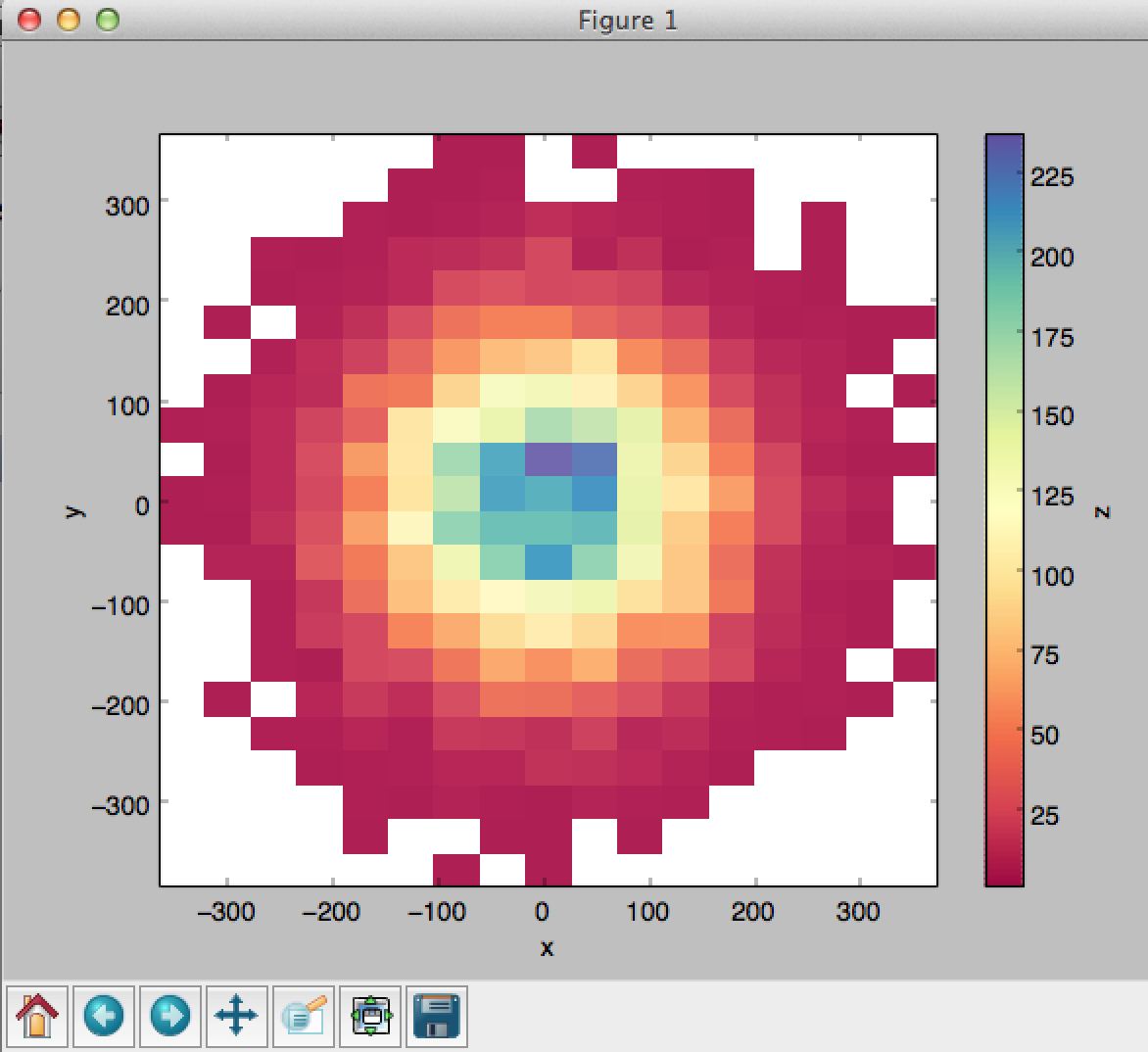
A. Yes. Q. I obtained a very small bin width, which is likely to be erroneous. Why? A. You probably searched bin widths smaller than the sampling resolution of your data. Please begin the search from the bin width as large as your sampling resolution. The minimum binwidth that the web-app searches is your data range divided by 200. If your sampling resolution is larger than it, ignore the suggested optimal bin. Please find the minimum in the cost function in `datasheet' for the bins larger than your sampling resolution. Q. Can I apply the method to the data composed of integer values? A. Yes. Please note that the resolution of your data is an integer. It is recommended to search only the bin widths which are a multiple of the resolution of your sampled data. Do not search the bin width smaller than the resolution. (The current version of web application can NOT be used for computing only integer bin widths.) Q. I obtained a large bin-width even if relatively large number of samples ~1000 are used. A. If you made a program by yourself, please double check that the variance, v, in the formula was correctly computed. It is a biased variance of event counts of a histogram. Please do not use an unbiased variance which uses N-1 to divides the sum of squared errors. A built-in function for variance calculation in a software may returns unbiased variance as a default. Q. I want to make a 2-dimensional histogram. Can I use this method? A. Yes. The same formula can be used for optimizing 2d histogram. The 'bin size' of a 2d histogram is the area of a segmented square cell. The mean and the variance are simply computed from the event counts in all the bins of the 2-dimensional histogram. Matlab sample program for selecting bin size of 2-d histogram. Python sample program (contribution by Cristóvão Freitas Iglesias Junior)
(The current version of web application can NOT be used for computing 2-dimensional histogram.) See also 2-d kernel density estimation Q. I have used the Scott's method Optimal Bin Size= 3.49*s*n^(-1/3) ,
and obtained bin size that differs from the result obtained by the
present method.
A. They should be different. Three assumptions were made to obtain the Scott's result. First, the Scott's result is asymptotically true (i.e. it is true for large sample size n). Second, the scaling exponent -1/3 is true if the density is a smooth function. Third, the coefficient 3.49 was obtained, assuming the Gauss density function as a reference. The present method does not require these assumptions. Q.What is the assumption in your method? A. The method only assumes that the data are sampled independently each other (an assumption of a Poisson point process). No assumption was made for the underlying density function (for example, unimodality, continuity, existence of derivatives, etc.). Q. Is it different from the least squares cross-validation method? A. Yes. The above formula was derived under a Poisson point process assumption [see original paper], not by the cross-validation. As a result, the formulas and chosen bandwidths by the two methods are not identical. Q. What is specific about the Poisson assumption? A. In classical density estimation, the sampling size is fixed. Under the Poisson assumption, the total data size is not fixed, but assumed to obey a Poisson distribution. The MISE is an average error measured by the histograms with 'many' realizations of the experiment. Hence, the histograms constructed from a Poisson point events have more variability than the histograms constructed from samples with a fixed amount. This leads to a choice of wider optimal bin size for a histogram under a Poisson point process assumption. The difference becomes negligible as we increase the data size. Q. You provide the method for optimizing kernel density estimate, too. Which of the methods, a histogram or kernel, do you recommend for density estimation? A. We generally recommend to use the kernel density estimate. Please check the kernel density optimization page, too.
The FAQ includes my (HS) opinion. They are not opinions neither by my collaborators nor institutions I belong to. |
How it works
|
A bar-graph histogram is constructed simply by counting the
number of events that belong to each bin of width In this thesis, we assess the goodness of the fit of the
estimator
By segmenting the range
The second term of Eq.(3.5) can further be decomposed into two parts,
By replacing
|
Code
YOUR CONTRIBUTION WELCOME! The codes include contribution by scientists from all over the world. If you could improve the code or translate the code to other languages, e.g., C/C++, please contact |
A Sample Matlab Program
|
The matlab function sshist.m
is now available. [2008/11/19]
Below is a simple sample program. %%%%%%%%%%%%%%%%%%%%%%%%%%%%%%%%%%%%%%%%%%%%%%%%%%%%%%%%%%%%%%%%%%
% 2006 Author Hideaki Shimazaki
% Department of Physics, Kyoto University
% shimazaki at ton.scphys.kyoto-u.ac.jp
% Please feel free to use/modify this program.
%
% Data: the duration for eruptions of
% the Old Faithful geyser in Yellowstone National Park (in minutes)
clear all;
x = [4.37 3.87 4.00 4.03 3.50 4.08 2.25 4.70 1.73 4.93 1.73 4.62 ...
3.43 4.25 1.68 3.92 3.68 3.10 4.03 1.77 4.08 1.75 3.20 1.85 ...
4.62 1.97 4.50 3.92 4.35 2.33 3.83 1.88 4.60 1.80 4.73 1.77 ...
4.57 1.85 3.52 4.00 3.70 3.72 4.25 3.58 3.80 3.77 3.75 2.50 ...
4.50 4.10 3.70 3.80 3.43 4.00 2.27 4.40 4.05 4.25 3.33 2.00 ...
4.33 2.93 4.58 1.90 3.58 3.73 3.73 1.82 4.63 3.50 4.00 3.67 ...
1.67 4.60 1.67 4.00 1.80 4.42 1.90 4.63 2.93 3.50 1.97 4.28 ...
1.83 4.13 1.83 4.65 4.20 3.93 4.33 1.83 4.53 2.03 4.18 4.43 ...
4.07 4.13 3.95 4.10 2.27 4.58 1.90 4.50 1.95 4.83 4.12];
x_min = min(x);
x_max = max(x);
N_MIN = 4; % Minimum number of bins (integer)
% N_MIN must be more than 1 (N_MIN > 1).
N_MAX = 50; % Maximum number of bins (integer)
N = N_MIN:N_MAX; % # of Bins
D = (x_max - x_min) ./ N; % Bin Size Vector
%%%%%%%%%%%%%%%%%%%%%%%%%%%%%%%%%%%%%%%%%%%%%%%%%%%%%%%%%%%%%%%%%%
% Computation of the Cost Function
for i = 1: length(N)
edges = linspace(x_min,x_max,N(i)+1); % Bin edges
ki = histc(x,edges); % Count # of events in bins
ki = ki(1:end-1);
k = mean(ki); % Mean of event count
v = sum( (ki-k).^2 )/N(i); % Variance of event count
C(i) = ( 2*k - v ) / D(i)^2; % The Cost Function
end
%%%%%%%%%%%%%%%%%%%%%%%%%%%%%%%%%%%%%%%%%%%%%%%%%%%%%%%%%%%%%%%%%%
% Optimal Bin Size Selectioin
[Cmin idx] = min(C);
optD = D(idx); % *Optimal bin size
edges = linspace(x_min,x_max,N(idx)+1); % Optimal segmentation
%%%%%%%%%%%%%%%%%%%%%%%%%%%%%%%%%%%%%%%%%%%%%%%%%%%%%%%%%%%%%%%%%%
% Display an Optimal Histogram and the Cost Function
subplot(1,2,1); hist(x,edges); axis square;
subplot(1,2,2); plot(D,C,'k.',optD,Cmin,'r*'); axis square;
|
A Sample R Program
Copy and Paste a sample program sample.R, then run sshist(faithful[,1]) . Display code close
#%%%%%%%%%%%%%%%%%%%%%%%%%%%%%%%%%%%%%%%%%%%%%%%%%%%%%%%%%%%%%%%%%
# 2006 Author Hideaki Shimazaki
# Department of Physics, Kyoto University
# shimazaki at ton.scphys.kyoto-u.ac.jp
sshist <- function(x){

	N <- 2: 100
	C <- numeric(length(N))
	D <- C

	for (i in 1:length(N)) {
		D[i] <- diff(range(x))/N[i]

		edges = seq(min(x),max(x),length=N[i])
		hp <- hist(x, breaks = edges, plot=FALSE )
		ki <- hp$counts

		k <- mean(ki)
		v <- sum((ki-k)^2)/N[i]

		C[i] <- (2*k-v)/D[i]^2	#Cost Function
	}

	idx <- which.min(C)
	optD <- D[idx]

	edges <- seq(min(x),max(x),length=N[idx])
	h = hist(x, breaks = edges )
	rug(x)

	return(h)
}
|
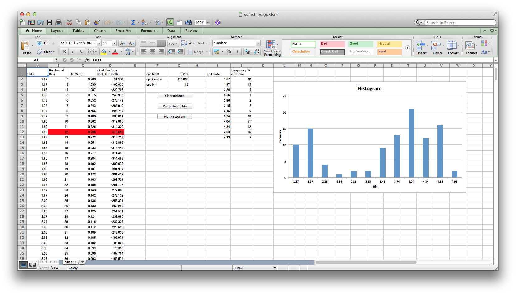
An Excel Program (contribution by Anil Kumar Tyagi)
 |
Sample Python Programs for 1D histogram
(contribution by Érbet Almeida Costa and Takuma Torii )
"""
Created on Thu Oct 25 11:32:47 2012

Histogram Binwidth Optimization Method

Shimazaki and Shinomoto, Neural Comput 19 1503-1527, 2007
2006 Author Hideaki Shimazaki, Matlab
Department of Physics, Kyoto University
shimazaki at ton.scphys.kyoto-u.ac.jp
Please feel free to use/modify this program.

Version in python adapted Érbet Almeida Costa

Data: the duration for eruptions of
the Old Faithful geyser in Yellowstone National Park (in minutes)
or normal distribuition.
Version in python adapted Érbet Almeida Costa
Bugfix by Takuma Torii 2.24.2013

"""

import numpy as np
from numpy import mean, size, zeros, where, transpose
from numpy.random import normal
from matplotlib.pyplot import hist
from scipy import linspace
import array

from matplotlib.pyplot import figure,  plot, xlabel, ylabel,\
    title, show, savefig, hist

x = normal(0, 100, 1e2) # Generate n pseudo-random numbers whit(mu,sigma,n)
#x = [4.37,3.87,4.00,4.03,3.50,4.08,2.25,4.70,1.73,4.93,1.73,4.62,\
#3.43,4.25,1.68,3.92,3.68,3.10,4.03,1.77,4.08,1.75,3.20,1.85,\
#4.62,1.97,4.50,3.92,4.35,2.33,3.83,1.88,4.60,1.80,4.73,1.77,\
#4.57,1.85,3.52,4.00,3.70,3.72,4.25,3.58,3.80,3.77,3.75,2.50,\
#4.50,4.10,3.70,3.80,3.43,4.00,2.27,4.40,4.05,4.25,3.33,2.00,\
#4.33,2.93,4.58,1.90,3.58,3.73,3.73,1.82,4.63,3.50,4.00,3.67,\
#1.67,4.60,1.67,4.00,1.80,4.42,1.90,4.63,2.93,3.50,1.97,4.28,\
#1.83,4.13,1.83,4.65,4.20,3.93,4.33,1.83,4.53,2.03,4.18,4.43,\
#4.07,4.13,3.95,4.10,2.27,4.58,1.90,4.50,1.95,4.83,4.12]

x_max = max(x)
x_min = min(x)
N_MIN = 4   #Minimum number of bins (integer)
            #N_MIN must be more than 1 (N_MIN > 1).
N_MAX = 50  #Maximum number of bins (integer)
N = range(N_MIN,N_MAX) # #of Bins
N = np.array(N)
D = (x_max-x_min)/N    #Bin size vector
C = zeros(shape=(size(D),1))

#Computation of the cost function
for i in xrange(size(N)):
    edges = linspace(x_min,x_max,N[i]+1) # Bin edges
    ki = hist(x,edges) # Count # of events in bins
    ki = ki[0]
    k = mean(ki) #Mean of event count
    v = sum((ki-k)**2)/N[i] #Variance of event count
    C[i] = (2*k-v)/((D[i])**2) #The cost Function
#Optimal Bin Size Selection

cmin = min(C)
idx  = where(C==cmin)
idx = int(idx[0])
optD = D[idx]

edges = linspace(x_min,x_max,N[idx]+1)
fig = figure()
ax = fig.add_subplot(111)
ax.hist(x,edges)
title(u"Histogram")
ylabel(u"Frequency")
xlabel(u"Value")
savefig('Hist.png')
fig = figure()
plot(D,C,'.b',optD,cmin,'*r')
savefig('Fobj.png')
|
A Sample Python Program for 2D histogram
(contribution by Cristóvão Freitas Iglesias Junior)
|
A Sample Mathematica Program
Copy and Paste a sample program sample.nb, then ctrl+shift. Display code close |
IDL Functions (contribution by Dr. Shigenobu Hirose)
|
The following IDL programs were contributed by Dr. Shigenobu Hirose at JAMSTEC. sshist.pro 1-dimensional histogram optimization. Display code close
sshist_2d.pro 2-dimensional histogram optimization. Display code close
|
Java program
|
The web appliation is written in Java. Here are the core codes, BinSelection.java and DrawHistogram.java . (BarHisto.java) They work with Javascript on this page. |
Links
|
Other applications for analyzing spike data: SULAB ( Prof. Shinomoto ) |
© 2006-11 Hideaki Shimazaki All rights reserved.